data_color: Perform data cell colorization

Description

It's possible to add color to data cells according to their values with the data_color() function. There is a multitude of ways to perform data cell colorizing here:

targeting: we can constrain which columns and rows should receive the colorization treatment (through the columns and rows arguments)
direction: ordinarily we perform coloring in a column-wise fashion but there is the option to color data cells in a row-wise manner (this is controlled by the direction argument)
coloring method: data_color() automatically computes colors based on the column type but you can choose a specific methodology (e.g., with bins or quantiles) and the function will generate colors accordingly; the method argument controls this through keywords and other arguments act as inputs to specific methods
coloring function: a custom function can be supplied to the fn argument for finer control over color evaluation with data; the color mapping col_*() functions in the scales package can be used here or any function you might want to define
color palettes: with palette we could supply a vector of colors, a virdis or RColorBrewer palette name, or, a palette from the paletteer package
value domain: we can either opt to have the range of values define the domain, or, specify one explicitly with the domain argument
indirect color application: it's possible to compute colors from one column and apply them to one or more different columns; we can even perform a color mapping from multiple source columns to the same multiple of target columns
color application: with the apply_to argument, there's an option for whether to apply the cell-specific colors to the cell background or the cell text
text autocoloring: if colorizing the cell background, data_color() will automatically recolor the foreground text to provide the best contrast (can be deactivated with autocolor_text = FALSE)

The data_color() function won't fail with the default options used, but that won't typically provide you the type of colorization you really need. You can however safely iterate through a collection of different options without running into too many errors.

Usage

data_color(
  data,
  columns = everything(),
  rows = everything(),
  direction = c("column", "row"),
  target_columns = NULL,
  method = c("auto", "numeric", "bin", "quantile", "factor"),
  palette = NULL,
  domain = NULL,
  bins = 8,
  quantiles = 4,
  levels = NULL,
  ordered = FALSE,
  na_color = NULL,
  alpha = NULL,
  reverse = FALSE,
  fn = NULL,
  apply_to = c("fill", "text"),
  autocolor_text = TRUE,
  contrast_algo = c("apca", "wcag"),
  colors = NULL
)

Value

An object of class gt_tbl.

Arguments

data: A table object that is created using the gt() function.
columns, rows: The columns and rows to which cell data color operations are constrained.
direction: Should the color computations be performed column-wise or row-wise? By default this is set with the "column" keyword and colors will be applied down columns. The alternative option with the "row" keyword ensures that the color mapping works across rows.
target_columns: For indirect column coloring treatments, we can supply the columns that will receive the styling. The necessary precondition is that we must use direction = "column". If columns resolves to a single column then we may use one or more columns in target_columns. If on the other hand columns resolves to multiple columns, then target_columns must resolve to the same multiple.
method: A method for computing color based on the data within body cells. Can be "auto" (the default), "numeric", "bin", "quantile", or "factor". The "auto" method will automatically choose the "numeric" method for numerical input data or the "factor" method for any non-numeric inputs.
palette: A vector of color names, the name of an RColorBrewer palette, the name of a viridis palette, or a discrete palette accessible from the paletteer package using the <package>::<palette> syntax (e.g., "wesanderson::IsleofDogs1"). If providing a vector of colors as a palette, each color value provided must either be a color name (Only R/X11 color names or CSS 3.0 color names) or a hexadecimal string in the form of "#RRGGBB" or "#RRGGBBAA". If nothing is provided here, the default R color palette is used (i.e., the colors from palette()).
domain: The possible values that can be mapped. For the "numeric" and "bin" methods, this can be a numeric range specified with a length of two vector. Representative numeric data is needed for the "quantile" method and categorical data must be used for the "factor" method. If NULL (the default value), the values in each column or row (depending on direction) value will represent the domain.
bins: For method = "bin" this can either be a numeric vector of two or more unique cut points, or, a single numeric value (greater than or equal to 2) giving the number of intervals into which the domain values are to be cut. By default, this is 8.
quantiles: For method = "quantile" this is the number of equal-size quantiles to use. By default, this is set to 4.
levels: For method = "factor" this allows for an alternate way of specifying levels. If anything is provided here then any value supplied to domain will be ignored. This should be a character vector of unique values.
ordered: For method = "factor", setting this to TRUE means that the vector supplied to domain will be treated as being in the correct order if that vector needs to be coerced to a factor. By default, this is FALSE.
na_color: The color to use for missing values. By default (with na_color = NULL) gray, "#808080", will be used.
alpha: An optional, fixed alpha transparency value that will be applied to all of the colors provided (regardless of whether a color palette was directly supplied or generated through a color mapping function).
reverse: Should the colors computed operate in reverse order? If TRUE then colors that normally change from red to blue will change in the opposite direction. By default, this is FALSE.
fn: A color-mapping function. The function should be able to take a vector of data values as input and return an equal-length vector of color values. The col_*() functions provided in the scales package (i.e., scales::col_numeric(), scales::col_bin(), and scales::col_factor()) can be invoked here with options, as those functions themselves return a color-mapping function.
apply_to: Which style element should the colors be applied to? Options include the cell background (the default, given as "fill") or the cell text ("text").
autocolor_text: An option to let gt modify the coloring of text within cells undergoing background coloring. This will result in better text-to-background color contrast. By default, this is set to TRUE.
contrast_algo: The color contrast algorithm to use when autocolor_text = TRUE. By default this is "apca" (Accessible Perceptual Contrast Algorithm) and the alternative to this is "wcag" (Web Content Accessibility Guidelines).
colors: Deprecated. Use the fn argument instead to provide a scales-based color-mapping function. If providing a palette, use the palette argument.

Targeting cells with <code>columns</code> and <code>rows</code>

Targeting of values is done through columns and additionally by rows (if nothing is provided for rows then entire columns are selected). The columns argument allows us to target a subset of cells contained in the resolved columns. We say resolved because aside from declaring column names in c() (with bare column names or names in quotes) we can use tidyselect-style expressions. This can be as basic as supplying a select helper like starts_with(), or, providing a more complex incantation like

where(~ is.numeric(.x) && max(.x, na.rm = TRUE) > 1E6)

which targets numeric columns that have a maximum value greater than 1,000,000 (excluding any NAs from consideration).

By default all columns and rows are selected (with the everything() defaults). Cell values that are incompatible with a given coloring function/method will be skipped over. One strategy is to color the bulk of cell values with one formatting function and then constrain the columns for later passes (the last coloring done to a cell is what you get in the final output).

Once the columns are targeted, we may also target the rows within those columns. This can be done in a variety of ways. If a stub is present, then we potentially have row identifiers. Those can be used much like column names in the columns-targeting scenario. We can use simpler tidyselect-style expressions (the select helpers should work well here) and we can use quoted row identifiers in c(). It's also possible to use row indices (e.g., c(3, 5, 6)) though these index values must correspond to the row numbers of the input data (the indices won't necessarily match those of rearranged rows if row groups are present). One more type of expression is possible, an expression that takes column values (can involve any of the available columns in the table) and returns a logical vector. This is nice if you want to base formatting on values in the column or another column, or, you'd like to use a more complex predicate expression.

Color computation methods

The data_color() function offers four distinct methods for computing color based on cell data values. They are set by the method argument and the options go by the keywords "numeric", "bin", "quantile", and "factor". There are other arguments in data_color() that variously support these methods (e.g., bins for the "bin" method, etc.). Here we'll go through each method, providing a short explanation of what each one does and which options are available.

`"numeric"`

The "numeric" method provides a simple linear mapping from continuous numeric data to an interpolated palette. Internally, this uses the scales::col_numeric() function. This method is suited for numeric data cell values and can make use of a supplied domain value, in the form of a two-element numeric vector describing the range of values, if provided.

`"bin"`

The "bin" method provides a mapping of continuous numeric data to value-based bins. Internally, this uses the scales::col_bin() function which itself uses base::cut(). As with the "numeric" method, "bin" is meant for numeric data cell values. The use of a domain value is supported with this method. The bins argument in data_color() is specific to this method, offering the ability to: (1) specify the number of bins, or (2) provide a vector of cut points.

`"quantile"`

The "quantile" method provides a mapping of continuous numeric data to quantiles. Internally, this uses the scales::col_quantile() function which itself uses stats::quantile(). Input data cell values should be numeric, as with the "numeric" and "bin" methods. A numeric domain value is supported with this method. The quantiles argument in data_color() controls the number of equal-size quantiles to use.

`"factor"`

The "factor" method provides a mapping of factors to colors. With discrete palettes, color interpolation is used when the number of factors does not match the number of colors in the palette. Internally, this uses the scales::col_factor() function. Input data cell values can be of any type (i.e., factor, character, numeric values, and more are supported). The optional input to domain should take the form of categorical data. The levels and ordered arguments in data_color() support this method.

Color palette access from RColorBrewer and viridis

All palettes from the RColorBrewer package and select palettes from viridis can be accessed by providing the palette name in palette. RColorBrewer has 35 available palettes:

	Palette Name	Colors	Category	Colorblind Friendly
1	`"BrBG"`	11	Diverging	Yes
2	`"PiYG"`	11	Diverging	Yes
3	`"PRGn"`	11	Diverging	Yes
4	`"PuOr"`	11	Diverging	Yes
5	`"RdBu"`	11	Diverging	Yes
6	`"RdYlBu"`	11	Diverging	Yes
7	`"RdGy"`	11	Diverging	No
8	`"RdYlGn"`	11	Diverging	No
9	`"Spectral"`	11	Diverging	No
10	`"Dark2"`	8	Qualitative	Yes
11	`"Paired"`	12	Qualitative	Yes
12	`"Set1"`	9	Qualitative	No
13	`"Set2"`	8	Qualitative	Yes
14	`"Set3"`	12	Qualitative	No
15	`"Accent"`	8	Qualitative	No
16	`"Pastel1"`	9	Qualitative	No
17	`"Pastel2"`	8	Qualitative	No
18	`"Blues"`	9	Sequential	Yes
19	`"BuGn"`	9	Sequential	Yes
20	`"BuPu"`	9	Sequential	Yes
21	`"GnBu"`	9	Sequential	Yes
22	`"Greens"`	9	Sequential	Yes
23	`"Greys"`	9	Sequential	Yes
24	`"Oranges"`	9	Sequential	Yes
25	`"OrRd"`	9	Sequential	Yes
26	`"PuBu"`	9	Sequential	Yes
27	`"PuBuGn"`	9	Sequential	Yes
28	`"PuRd"`	9	Sequential	Yes
29	`"Purples"`	9	Sequential	Yes
30	`"RdPu"`	9	Sequential	Yes
31	`"Reds"`	9	Sequential	Yes
32	`"YlGn"`	9	Sequential	Yes
33	`"YlGnBu"`	9	Sequential	Yes
34	`"YlOrBr"`	9	Sequential	Yes
35	`"YlOrRd"`	9	Sequential	Yes

We can access four colorblind-friendly palettes from viridis: "viridis", "magma", "plasma", and "inferno". Simply provide any one of those names to palette.

Color palette access from paletteer

Choosing the right color palette can often be difficult because it's both hard to discover suitable palettes and then obtain the vector of colors. To make this process easier we can elect to use the paletteer package, which makes a wide range of palettes from various R packages readily available. The info_paletteer() information table allows us to easily inspect all of the discrete color palettes available in paletteer. We only then need to specify the palette and associated package using the <package>::<palette> syntax (e.g., "tvthemes::Stannis") for the palette argument.

A requirement for using paletteer in this way is that the package must be installed (gt doesn't import paletteer currently). This can be easily done with install.packages("paletteer"). Not having this package installed with result in an error when using the <package>::<palette> syntax in palette.

Foreground text and background fill

By default, gt will choose the ideal text color (for maximal contrast) when colorizing the background of data cells. This option can be disabled by setting autocolor_text to FALSE. The contrast_algo argument lets us choose between two color contrast algorithms: "apca" (Accessible Perceptual Contrast Algorithm, the default algo) and "wcag" (Web Content Accessibility Guidelines).

Examples

The data_color() function can be used without any supplied arguments to colorize a gt table. Let's do this with the exibble dataset:

exibble |>
  gt() |>
  data_color()

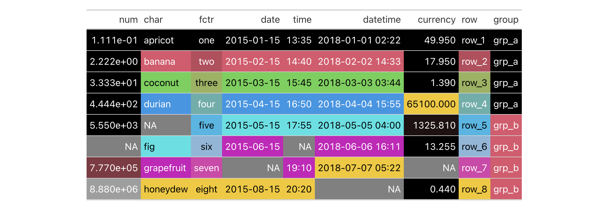
This image of a table was generated from the first code example in the `data_color()` help file.

What's happened is that data_color() applies background colors to all cells of every column with the default palette in R (accessed through palette()). The default method for applying color is "auto", where numeric values will use the "numeric" method and character or factor values will use the "factor" method. The text color will be undergo modification automatically to maximize contrast (since autocolor_text is TRUE by default).

You can use any of the available method keywords and gt will only apply color to the compatible values. Let's use the "numeric" method and supply palette values of "red" and "green".

exibble |>
  gt() |>
  data_color(
    method = "numeric",
    palette = c("red", "green")
  )

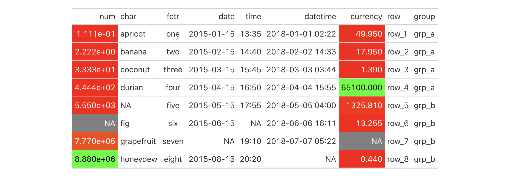
This image of a table was generated from the second code example in the `data_color()` help file.

With those options in place we see that only the numeric columns num and currency received color treatments. Moreover, the palette colors were mapped to the lower and upper limits of the data in each column; interpolated colors were used for the values in between the numeric limits of the two columns.

We can constrain the cells to which coloring will be applied with the columns and rows arguments. Further to this, we can manually set the limits of the data with the domain argument (which is preferable in most cases). Here, the domain will be set as domain = c(0, 50).

exibble |>
  gt() |>
  data_color(
    columns = currency,
    rows = currency < 50,
    method = "numeric",
    palette = c("red", "green"),
    domain = c(0, 50)
  )

This image of a table was generated from the third code example in the `data_color()` help file.

We can use any of the palettes available in the RColorBrewer and viridis packages. Let's make a new gt table from a subset of the countrypops dataset. Then, through data_color(), we'll apply coloring to the population column with the "numeric" method, use a domain between 2.5 and 3.4 million, and specify palette = "viridis".

countrypops |>
  dplyr::filter(country_name == "Mongolia") |>
  dplyr::select(-contains("code")) |>
  tail(10) |>
  gt() |>
  data_color(
    columns = population,
    method = "numeric",
    palette = "viridis",
    domain = c(2.5E6, 3.4E6)
  )

This image of a table was generated from the fourth code example in the `data_color()` help file.

We can alternatively use the fn argument for supplying the scales-based function scales::col_numeric(). That function call will itself return a function (which is what the fn argument actually requires) that takes a vector of numeric values and returns color values. Here is the more complex version of the code that returns the same table as in the previous example.

countrypops |>
  dplyr::filter(country_name == "Mongolia") |>
  dplyr::select(-contains("code")) |>
  tail(10) |>
  gt() |>
  data_color(
    columns = population,
    fn = scales::col_numeric(
      palette = "viridis",
      domain = c(2.5E6, 3.4E6)
    )
  )

This image of a table was generated from the fourth code example in the `data_color()` help file.

Using your own function in fn can be very useful if you want to make use of specialized arguments in the scales col_*() functions. You could even supply your own specialized function for performing complex colorizing treatments!

The data_color() function has a way to apply colorization indirectly to other columns. That is, you can apply colors to a column different from the one used to generate those specific colors. The trick is to use the target_columns argument. Let's do this with a more complete countrypops-based table example.

countrypops |>
  dplyr::filter(country_code_3 %in% c("FRA", "GBR")) |>
  dplyr::filter(year %% 10 == 0) |>
  dplyr::select(-contains("code")) |>
  dplyr::mutate(color = "") |>
  gt(groupname_col = "country_name") |>
  fmt_integer(columns = population) |>
  data_color(
    columns = population,
    target_columns = color,
    method = "numeric",
    palette = "viridis",
    domain = c(4E7, 7E7)
  ) |>
  cols_label(
    year = "",
    population = "Population",
    color = ""
  ) |>
  opt_vertical_padding(scale = 0.65)

This image of a table was generated from the fifth code example in the `data_color()` help file.

When specifying a single column in columns we can use as many target_columns values as we want. Let's make another countrypops-based table where we map the generated colors from the year column to all columns in the table. This time, the palette used is "inferno" (also from the viridis package).

countrypops |>
  dplyr::filter(country_code_3 %in% c("FRA", "GBR", "ITA")) |>
  dplyr::select(-contains("code")) |>
  dplyr::filter(year %% 5 == 0) |>
  tidyr::pivot_wider(
    names_from = "country_name",
    values_from = "population"
  ) |>
  gt() |>
  fmt_integer(columns = c(everything(), -year)) |>
  cols_width(
    year ~ px(80),
    everything() ~ px(160)
  ) |>
  opt_all_caps() |>
  opt_vertical_padding(scale = 0.75) |>
  opt_horizontal_padding(scale = 3) |>
  data_color(
    columns = year,
    target_columns = everything(),
    palette = "inferno"
  ) |>
  tab_options(
    table_body.hlines.style = "none",
    column_labels.border.top.color = "black",
    column_labels.border.bottom.color = "black",
    table_body.border.bottom.color = "black"
  )

This image of a table was generated from the sixth code example in the `data_color()` help file.

Now, it's time to use pizzaplace to create a gt table. The color palette to be used is the "ggsci::red_material" one (it's in the ggsci R package but also obtainable from the the paletteer package). Colorization will be applied to the to the sold and income columns. We don't have to specify those in columns because those are the only columns in the table. Also, the domain is not set here. We'll use the bounds of the available data in each column.

pizzaplace |>
  dplyr::group_by(type, size) |>
  dplyr::summarize(
    sold = dplyr::n(),
    income = sum(price),
    .groups = "drop_last"
  ) |>
  dplyr::group_by(type) |>
  dplyr::mutate(f_sold = sold / sum(sold)) |>
  dplyr::mutate(size = factor(
    size, levels = c("S", "M", "L", "XL", "XXL"))
  ) |>
  dplyr::arrange(type, size) |>
  gt(
    rowname_col = "size",
    groupname_col = "type"
  ) |>
  fmt_percent(
    columns = f_sold,
    decimals = 1
  ) |>
  cols_merge(
    columns = c(size, f_sold),
    pattern = "{1} ({2})"
  ) |>
  cols_align(align = "left", columns = stub()) |>
  data_color(
    method = "numeric",
    palette = "ggsci::red_material"
  )

This image of a table was generated from the seventh code example in the `data_color()` help file.

Colorization can occur in a row-wise manner. The key to making that happen is by using direction = "row". Let's use the sza dataset to make a gt table. Then, color will be applied to values across each 'month' of data in that table. This is useful when not setting a domain as the bounds of each row will be captured, coloring each cell with values relative to the range. The palette is "PuOr" from the RColorBrewer package (only the name here is required).

sza |>
  dplyr::filter(latitude == 20 & tst <= "1200") |>
  dplyr::select(-latitude) |>
  dplyr::filter(!is.na(sza)) |>
  tidyr::spread(key = "tst", value = sza) |>
  gt(rowname_col = "month") |>
  sub_missing(missing_text = "") |>
  data_color(
    direction = "row",
    palette = "PuOr",
    na_color = "white"
  )

This image of a table was generated from the eighth code example in the `data_color()` help file.

Notice that na_color = "white" was used, and this avoids the appearance of gray cells for the missing values (we also removed the "NA" text with sub_missing(), opting for empty strings).

Function ID

3-30

Function Introduced

v0.2.0.5 (March 31, 2020)